PTSP Example

This web page provide a full description of an PTSP example with detailed steps of the scheduling procedure to illustrate the article:

Philippe Lacomme, Aziz Moukrim, Alain Quilliot, Marina Vinot. Supply Chain Optimization with both Production and Transportation Integration: Multiple Vehicles for a Single Perishable Product. International Journal of Production Research. Accepted article

• The example:

Let us consider the result obtained by the Split (see more detailed ...) with 5 sub-trips using 3 vehicles. Having the production costs for the 5 sub-trips p = (6,2,4,8,3) and also the transportation costs t = (20,10,30,25,20) of each sub-trip and starting with a Bierwirth vector in the same order than the split procedure VB = [1,2,3,5,4].

At the first iteration, the algorithm adds into the graph, the disjunctive arc considering the job number 1 in first position into the vector and the job number 2 which is in second position. Since the operation 1 is assigned to the vehicle V1, and the operation 2 at the vehicle V2, only one disjunctive arc is added between the two production-operation and not between the two transport operations. In the third position into the vector VB, the job number 3 required the vehicle V3, only one disjunctive arc is added between the two production operations. Then the job number 4 is considered and two disjunctive arc are added. The first disjunctive arc is added from the production operation of the job 3 and the second disjunctive arc is added from the transport operation of the job 2 and the transport operation of the job 4 which required both the vehicle V2. And the job number 5 is added and two disjunctive arcs are added like before.

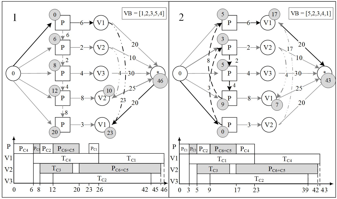
Fig 1: Detail of steps of the scheduling procedure with 5 sub-trips and V=3

This process is an extension of the initial Bierwirth's proposal, which is fully commonly described in numerous publications in job-shop or job-shop with extensions. At the end of process, the makespan is 46 and the solution is represented on Fig. 1 part 1. The first local search movement investigates the permutation of job 1 and 5 leading to a new neighborhood vector VB = [5,2,3,4,1] with a makespan equal to 43. The four next iterations of the local search provides four vectors VB = [5,2,3,1,4] with a makespan of 56, VB = [5,2,4,3,1] with a makespan of 49, VB = [5,3,2,4,1] with a makespan of 45 and the final vector is VB = [2,5,3,4,1] with a makespan of 45. The best solution was obtain at step 2 on Fig. 1 part 2 with a vector VB = [5,2,3,4,1] and a makespan equal to 43.