PTSP Example

This web page provide a full description of an PTSP example with detailed steps of the split procedure to illustrate the article:

Philippe Lacomme, Aziz Moukrim, Alain Quilliot, Marina Vinot. Supply Chain Optimization with both Production and Transportation Integration: Multiple Vehicles for a Single Perishable Product. International Journal of Production Research. Accepted article

• The example:

Let us consider one instance with 6 customers, 3 vehicles with a capacity equal to 10 and a product lifespan equal to 20 (Table 0). Table 1 provides the distance matrix, assuming a directed network (depot is numbered as 0). The giant tour to be split is GT=(4,3,2,6,5,1).

Table 0:

Instances:	Number of customers	Customers' demands qi	Number of vehicles	Capacity of vehicles Q	Lifespan of the product B
Example	6	{3;4;2;6;5;3}	3	10	20

Table 1:Distance matrix between customers

/	0	1	2	3	4	5	6
0	0	10	15	5	10	5	10
1	10	0	10	10	30	20	20
2	15	10	0	25	30	20	10
3	5	10	25	0	10	15	20
4	10	30	30	10	0	10	15
5	5	20	20	15	10	0	10
6	10	20	10	20	15	10	0

The initial label of node 0 is L=(0,0,0,0) and the arc (0,1) in the auxiliary graph corresponds to a sub-trip which encompasses only the customer 4 i.e. T₁=4, with q(T₁)=q₄=6. Since vehicles are identical, only one label is generated from the initial label using this arc leading to the following final label on node 1: P=(6,26,0,0). This label models a solution where the production of customer C4 is finished at time 6 and where the transport of customer is achieved at d_V1=6+20=26.

Fig. 1 represents the solution modelled by the label (6,26,0,0) obtained after propagation of the label (0,0,0,0) from node 0 to node 1. Fig. 2 gives the situation where the customers C4 and C3 are in the same sub-trip and modelled by the label (8,33,0,0) which has been created thanks to a propagation from the node 0 to the node 2.

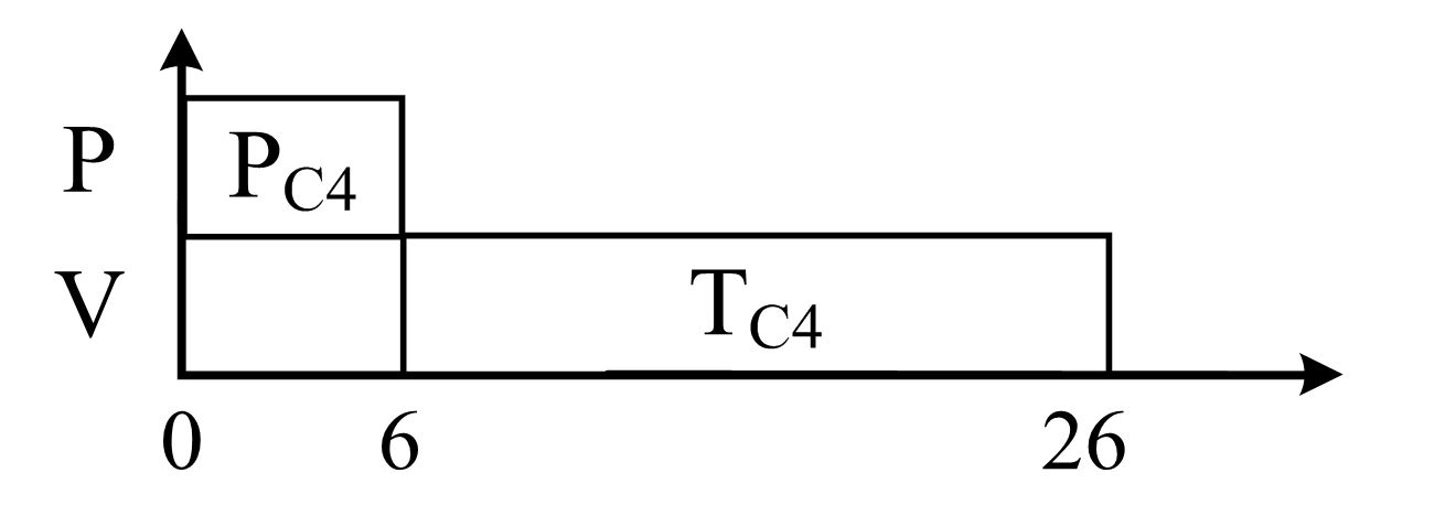
Fig 1: Customer 4 into one sub-trip (first propagation of the label(0,0,0,0))

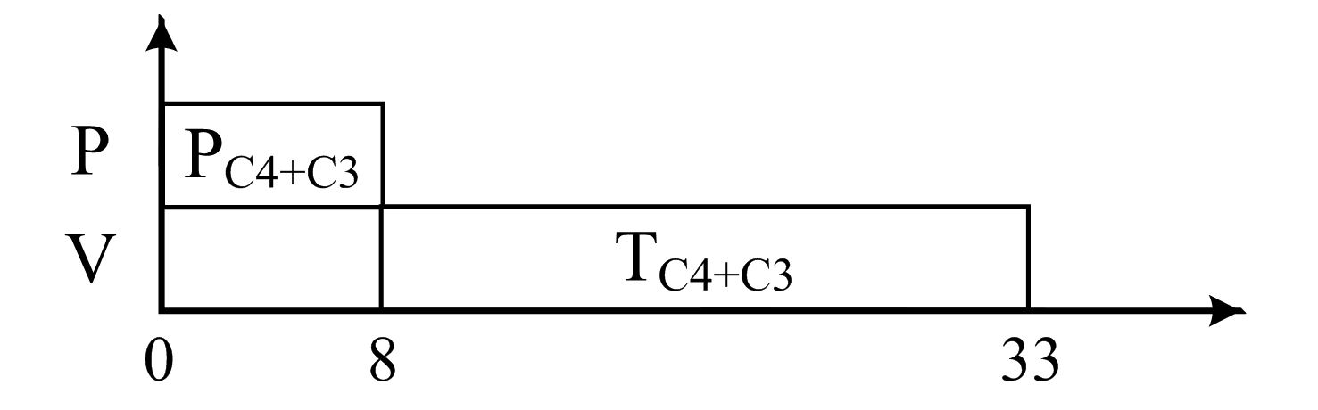
Fig 2: Customer 4 and 3 into one sub-trip (second propagation of the label(0,0,0,0))

Iteration of the process permits to obtain the label (6,26,0,0) on node 1 and one label on node 2 coming from node 0, label (8,33,0,0). Next the label (6,26,0,0) is propagated from node 1 to node 2 and leading to label (26,36,0,0) and label (8,26,18,0). This process is iterated to obtain a set of seven labels on node 3 where each label represents a specific solution (see Fig. 3).

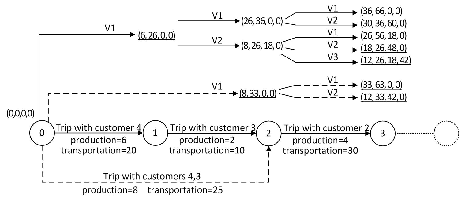
Fig 3: Example of labels generated by Split in the auxiliary graph

A label can create two quite different labels modeling strongly different solutions. Such a situation is explained on Fig. 4 which represents two solutions related to (33,63,0,0) and (12,33,42,0).

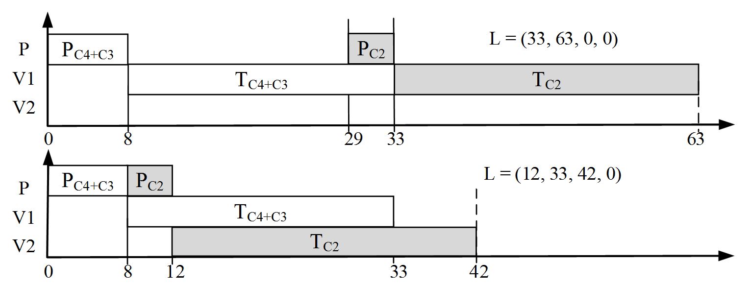
Fig 4: Propagation of label (8,33,0,0) from node 2 to node 3 on two different vehicles

The best solution obtained at the end of the Split is given by (26,46,45,42) on Fig. 5. The vehicles V₁,V₂,V₃,V₂,V₁ are used in this order and 5 sub-trips are build.

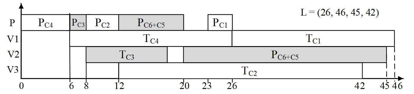
Fig 5: Final solution of the example