PCPSPR Example

This web page provide a full description of an RCPSPT example with detailed steps to illustrate the article:

Philippe Lacomme, Aziz Moukrim, Alain Quilliot, Marina Vinot. Integration of Routing into RCPSP. EURO Journal on Computational Optimization. Submitting article

• The example instance:   

Instances informations

The example presented in this page introduces an example of RCPSPT solution with 10 activities, each activity requiring a non-negative amount of the resource and has a duration(Table 1).

Table 0:

Instances:	Number of activities (starting and ending including)	Quantity of the resource available	Size of the square location of the activities	Number of vehicles	Capacities of vehicles C_u
LMQV_10	10	6	10 x 10	2	(3,2)

Table 1:

Activity:	Duration	Resources Requirement
0	0	/
1	10	2
2	15	2
3	20	2
4	30	2
5	10	3
6	30	2
7	20	3
8	10	3
9	0	/

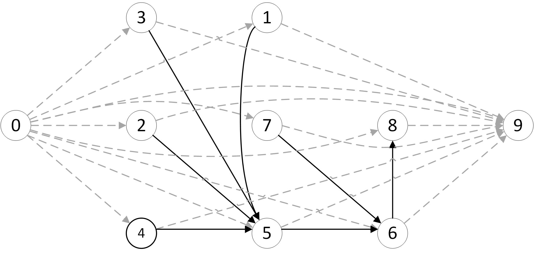
Fig 1: Precedence constraints of the example

The Fig. 1 models the precedence constraints between the activities and the Fig. 2 gives an example of resources quantities to be transferred to define a RCPSP solution. For example, activity 7 can be in progress only after receiving one unit of resource from activity 2 and 2 units of resource from activity 1.

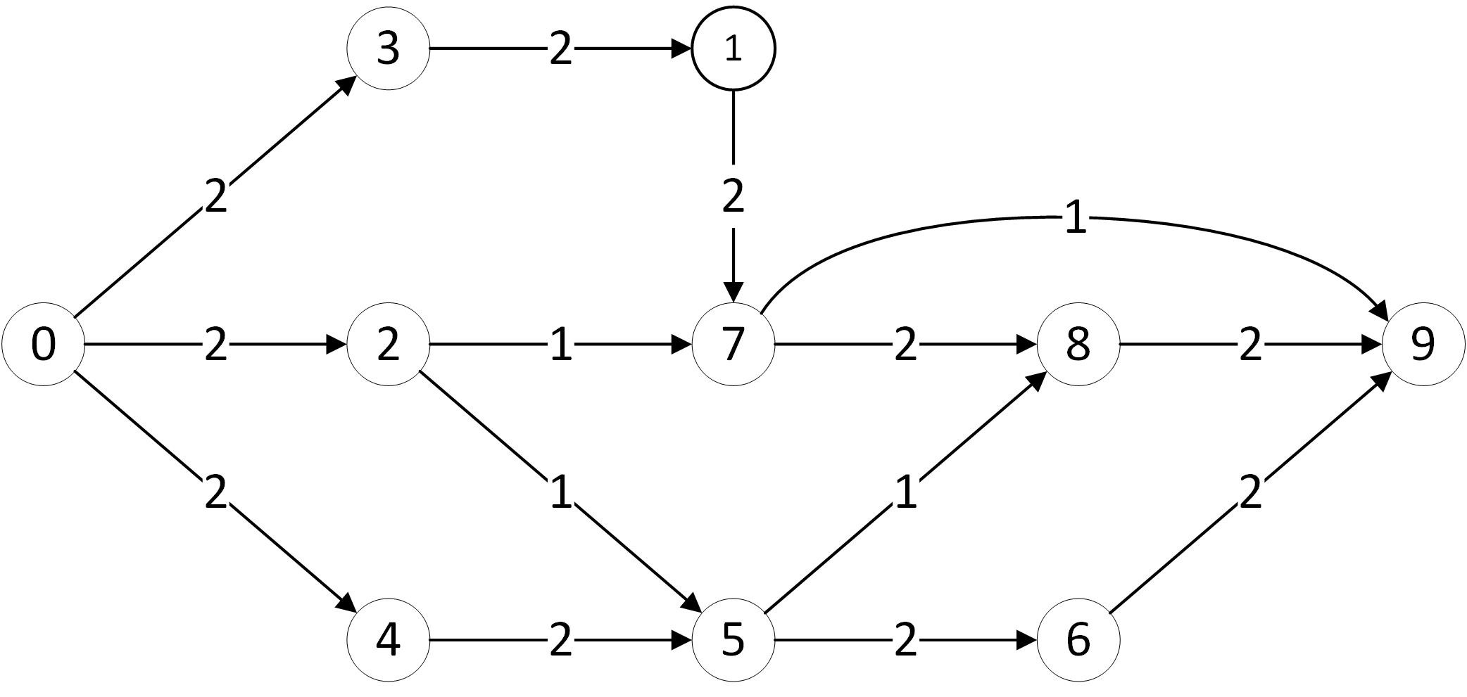
Fig 2: Example of resource transfer solution (flow)

A routing solution consists in assigning transportation operations to vehicles and to determine trips compliant with the resource transfer previously defined. The transport is achieved by a heterogeneous fleet of two vehicles of capacity 3 and 2 and the shortest path between activities is introduced in Table 2.The routing constraints will be added on the graph of Fig. 3 to obtain a RCPSPT solution. The Fig. 3 gather the constraints of the Fig. 1 and Fig. 2 to obtain a first disjunctive graph.

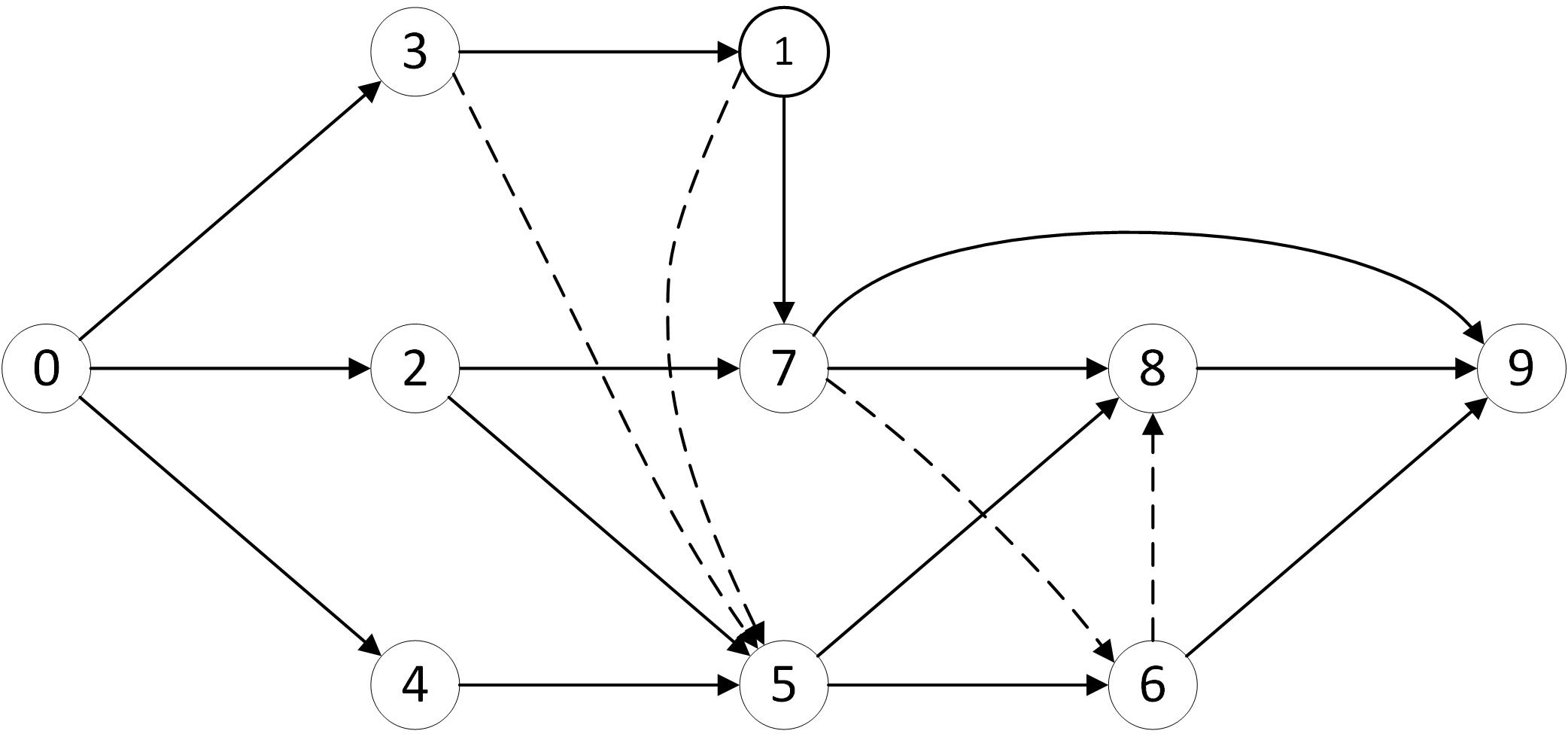
Fig 3: Example of disjunctive graph with disjunctions from the precedence constraints and the resource transfer

The transport operation can be modelled on the graph of Fig. 3 by adding squares on transfer arc to obtain a new graph (Fig.4).

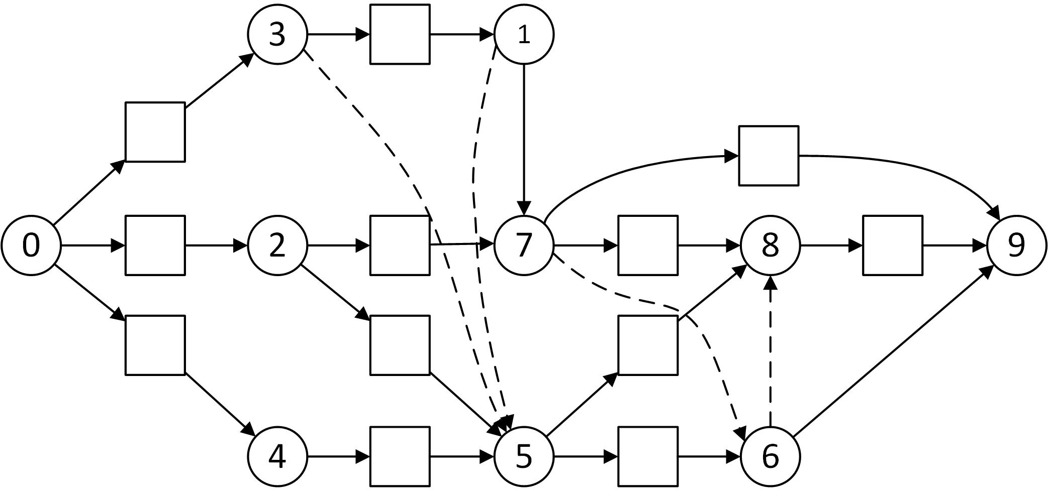
Fig 4: Disjunctive graph with the transport operation modelled but not enough assign

Table 2: Shortest path duration between activities of interest

/	0	1	2	3	4	5	6	7	8	9
0	0	3	4	3	10	13	12	8	11	12
1	3	0	3	4	11	14	13	6	9	10
2	4	3	0	3	14	17	16	9	12	13
3	3	4	3	0	13	16	15	10	13	14
4	10	11	14	13	0	3	4	9	11	9
5	13	14	17	16	3	0	3	10	12	9
6	12	13	16	15	4	3	0	8	9	6
7	8	6	9	10	9	4	3	0	3	4
8	11	9	12	13	11	12	9	3	0	3
9	12	10	13	14	9	9	8	4	4	0

The Gantt of Figure 5 defines a schedule by assigning activities to vehicle and determines the trips of vehicles which are composed of an ordered set of pickups and deliveries operations. The activity 4 is scheduled from time 10 to 40 (Fig. 5) and the earliest finishing time (which values 40) of activity 4 defines the exact time where the resources used by activity 4 are free to be transported from current position (in the unloaded buffer in rear of activity 4) to a new activity. Vehicle 1 is assigned to transport resources from depot to activity 4 with 2 units of resource and from activity 3 to 1 with 2 units of resource. Between this two successive loaded moves with two pickup/delivery operations, the vehicle achieves an unloaded move from position of activity 4 to position of activity 3.

Fig 4: Gantt solution with both scheduling and transport planning

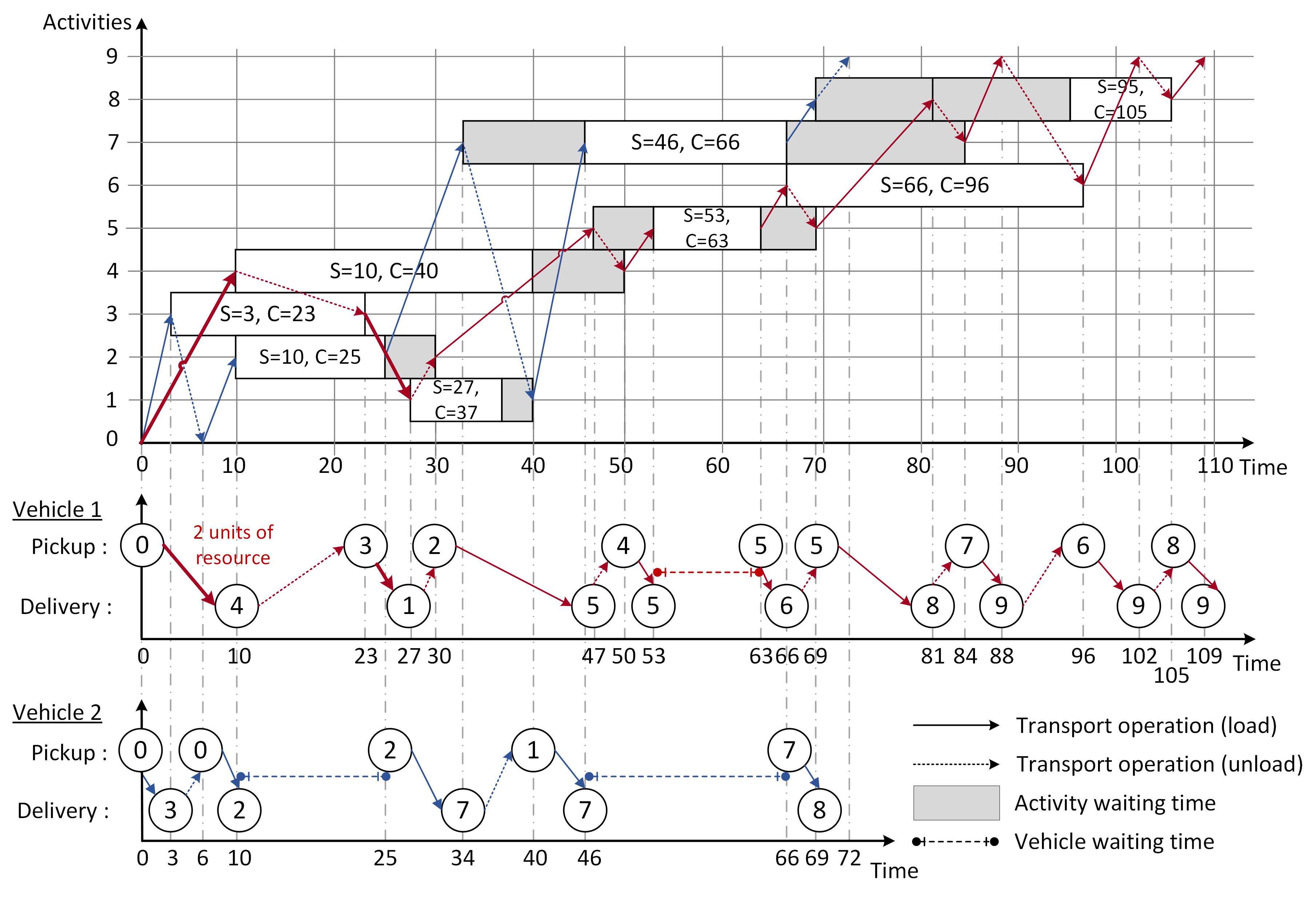
Each activity starting time and the completion time are reported in Table 3.

Table 3:

Activity:	Starting time	Completion time
0	0	0
1	27	37
2	10	25
3	3	23
4	10	40
5	53	63
6	66	96
7	46	66
8	96	106
9	109	109

By consequence, a full description of vehicle trip, is an ordered sequence of loaded transport operations (pickup/delivery transport) and unloaded transport operation. Table 4 gives a full description of vehicle 1 trip where the type of transport operation is L for loaded and U for unloaded. The first transport operation is a loaded transport operation from depot 0 to activity 4 with a vehicle departure time at 0 and a vehicle arrival time at 10  for a load of 2 units of resources. Between operation number 7 and 8 in trip 1, a waiting time of the vehicle on activity 5 can be noticed.

Table 4: Details of the two trips with all the transport operations

Trip1
Operation number	1	2	3	4	5	6	7		8	9	10	11	12	13	14	15	16
Transport  Operation	0-4	4-3	3-1	1-2	2-5	5-4	4-5	WT	5-6	6-5	5-8	8-7	7-9	9-6	6-9	9-8	8-9
Type	L	U	L	U	L	U	L		L	U	L	U	L	U	L	U	L
Departure time	0	10	23	27	30	47	50	/	63	66	69	81	84	88	96	102	105
Arrival time	10	23	27	30	47	50	53	/	66	69	81	84	88	96	102	105	109
Vehicle load	2	0	2	0	1	0	2	/	2	0	2	0	1	0	2	0	2
Waiting Time	/		/		/	/	/	10	/	/	/	/	/	/	/	/	/

Trip2
Operation number	1	2	3		4	5	6		7	8
Transport  Operation	0-3	3-0	0-2	WT	2-7	7-1	1-7	WT	7-8	8-9
Type	L	U	L		L	U	L		L	U
Departure time	0	3	6	/	25	34	40	/	66	69
Arrival time	3	6	10	/	34	40	46	/	69	72
Vehicle load	2	0	2	/	1	0	2	/	2	0
Waiting Time	/	/	/	10	/	/	/	20	/	/

Let us note that unloaded transport operations are also defined with a vehicle departure time and a vehicle arrival time which has been left shifted in the trip of Table 4.
The routing solution is a set of two trips and each trip is defined by an ordered sequence of transport operations with the departure time of the vehicle, the arrival time and the total amount of resources loaded. One transport operation is defined by an origin node where a pickup operation is achieved and a delivery node and the number of loaded resources. Because the resources required by an activity can be delivered by several loaded transports assigned to different vehicles, there is no partition of nodes between the vehicles and the graphical representation (Fig. 6) of the routing solution is quite different than the common DARP solutions.

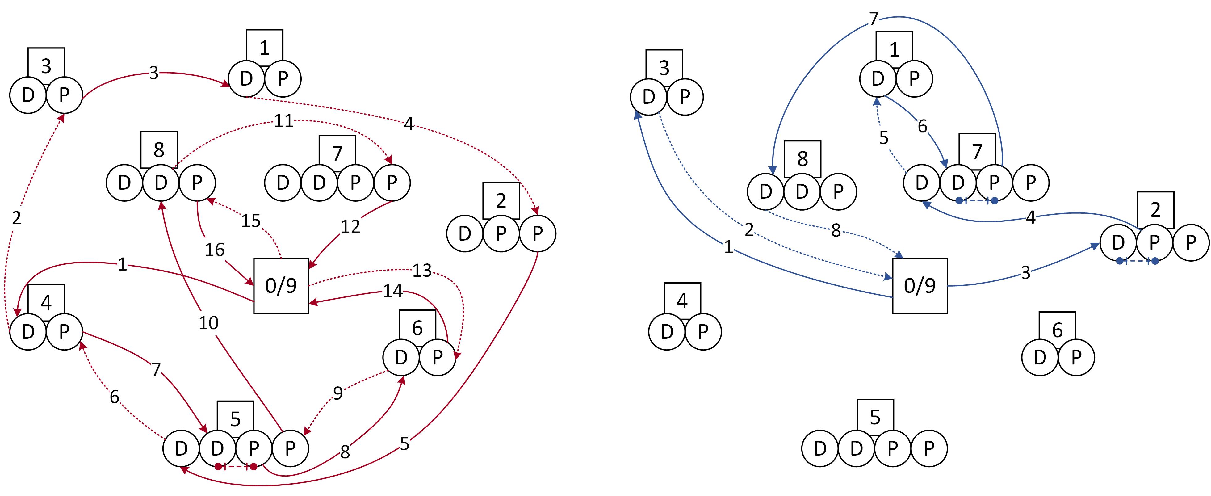Fig 5: Representation of the transport operations of trip 1 (left) and trip 2 (right)

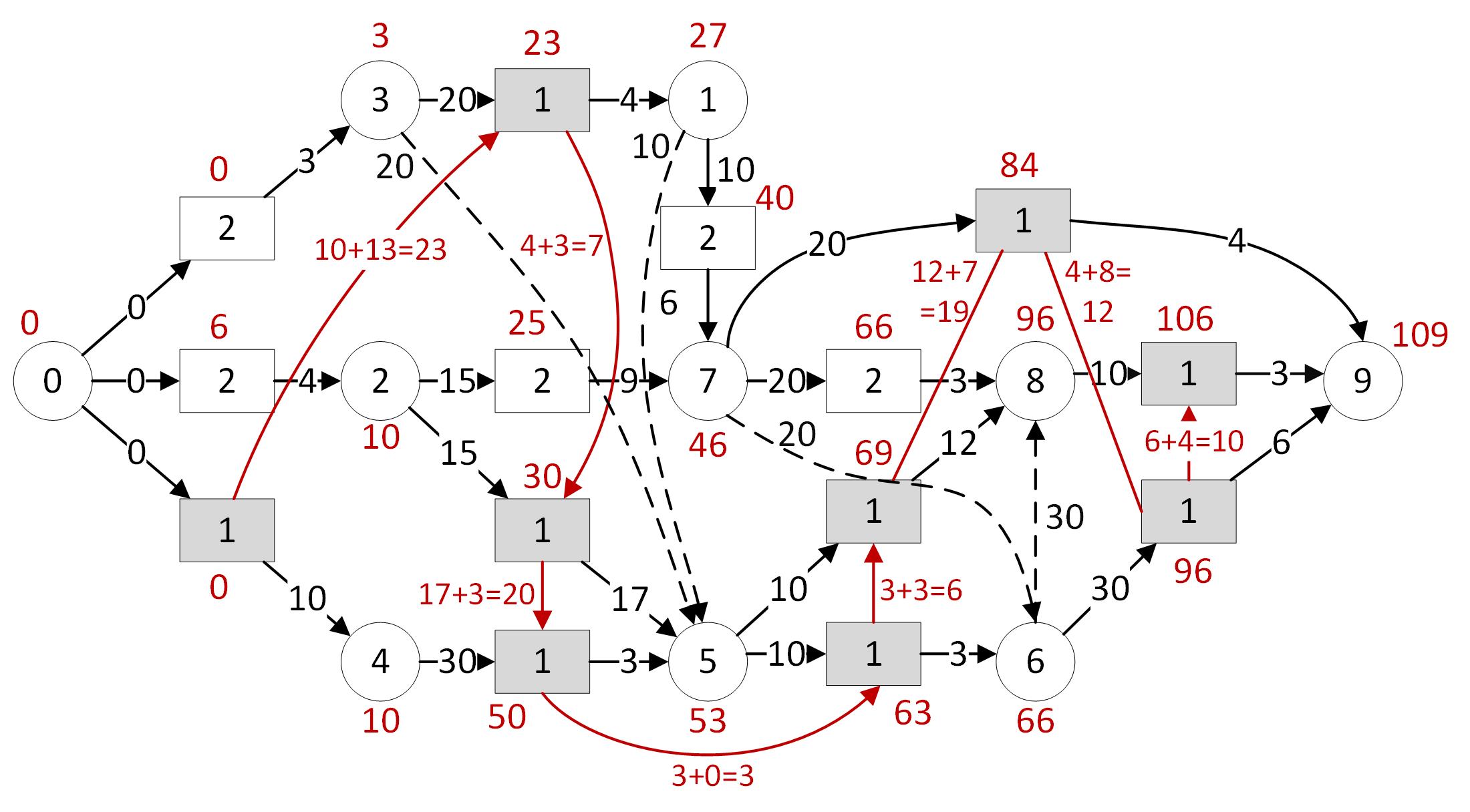Fig 6: Example of solution with a representation of the transport disjunction limited to vehicle 1