Hadoop Cluster

- MapReduce approach on one hadoop cluster for conception of new efficient optimization methods: application to the shortest path problem
- Published at Engineering Applications of Artificial Intelligence, Volume 41, May 2015, Pages 151-165. See it online
Authors | Instances | Results

Authors:

- Sabeur Aridhi
  
  Tel: +39 04 61 28 39 92
  Email: sabeur.aridhi@isima.fr
  Web page: http://fc.isima.fr/~aridhi/
  
  DISI, Department of Information Engineering and Computer Science, University of Trento
  Via Sommarive 9, 38123 Trento, Italy
- Philippe Lacomme
  
  Tel. : 04 73 40 75 85
  Email : placomme@isima.fr
  Web page: http://www.isima.fr/~lacomme/
  
  LIMOS - UMR CNRS 6158
  Universite Blaise Pascal
  Campus des Cezeaux, 63173 Aubiere CEDEX
- Libo Ren
  
  Tel. : 04 73 40 76 62
  Email : ren@isima.fr
  Web page: http://fc.isima.fr/~ren/
  
  LIMOS - UMR CNRS 6158
  Universite d'Auvergne
  Campus des Cezeaux, 63173 Aubiere CEDEX
- Benjamin Vincent
  
  Tel. : 04 73 40 77 72
  Email : benjamin.vincent@isima.fr
  
  LIMOS - UMR CNRS 6158
  Universite Blaise Pascal
  Campus des Cezeaux, 63173 Aubiere CEDEX

Instances:

Main characteristics

- based on large-scale real-road networks using OpenStreetMap data;
- 15 instances between french cities.

Data source

French real-road networks (OpenStreetMap data):

Http://download.geofabrik.de/europe/france.html
Subgraph download web service for French real-road networks (converted graph):

Local server Require a key

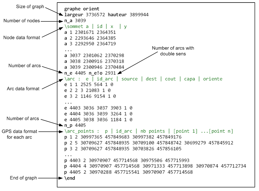
Subgraph format

Instances

Table. 1: Set of instances

	Origin		Destination
Instance	City	GPS position	City	GPS position
1	Clermont-Ferrand	45.779796 3.086371	Montluçon	46.340765 2.606664
2	Paris	48.858955 2.352934	Nice	43.70415 7.266376
3	Paris	48.858955 2.352934	Bordeaux	44.840899 -0.579729
4	Clermont-Ferrand	45.779796 3.086371	Bordeaux	44.840899 -0.579729
5	Lille	50.63569 3.062081	Toulouse	43.599787 1.431127
6	Brest	48.389888 -4.484496	Grenoble	45.180585 5.742559
7	Bayonne	43.494433 -1.482217	Brive-la-Gaillarde	45.15989 1.533916
8	Bordeaux	44.840899 -0.579729	Nancy	48.687334 6.179438
9	Grenoble	45.180585 5.742559	Bordeaux	44.840899 -0.579729
10	Reims	49.258759 4.030817	Montpellier	43.603765 3.877974
11	Reims	49.258759 4.030817	Dijon	47.322709 5.041509
12	Dijon	47.322709 5.041509	Lyon	45.749438 4.841852
13	Montpellier	43.603765 3.877974	Marseille	43.297323 5.369897
14	Perpignan	42.70133 2.894547	Reims	49.258759 4.030817
15	Rennes	48.113563 -1.66617	Strasbourg	48.582786 7.751825

All of the instances are based on the graph of road networks of France using OpenStreetMap data.
Download the OSM file

Results:

All experiments have been achieved on a hadoop cluster of 8 nodes corresponding to a set of homogenous computers connected through local area networks. Each computer is based on an AMD Opteron 2.3 GHz CPU under Linux (CentOS 64-bit). The number of cores used is set to 1 for all tests. The computational experiments have been achieved using hadoop 0.23.9.

Table 2. Comparison of results with 2 iterations

		D=15		D=30		D=50		D=100		D=150		D=200		Solutions download
Ins.	Opt.	Val.	Gap	Val.	Gap	Val.	Gap	Val.	Gap	Val.	Gap	Val.	Gap	Solutions download
1	87.1	96.8	11.11	92.3	5.95	87.1	0.00	87.1	0.00	87.1	0.00	87.1	0.00
2	841.2	-	-	-	-	934.7	11.12	908.7	8.02	854.7	1.60	850.5	1.09
3	537.4	574.3	6.87	557.7	3.78	549.5	2.25	542.4	0.93	542.0	0.85	537.4	0.00
4	355.6	381.6	7.31	375.1	5.49	369.6	3.95	361.5	1.67	355.6	0.00	358.0	0.68
5	883.8	954.4	7.99	933.2	5.59	926.4	4.82	912.9	3.29	913.1	3.31	908.7	2.82
6	948.2	1032.0	8.84	1007.5	6.25	989.6	4.37	971.8	2.48	970.3	2.33	965.1	1.78
7	349.6	377.0	7.85	372.4	6.55	361.8	3.51	356.1	1.88	352.4	0.81	349.6	0.00
8	750.1	814.3	8.56	792.5	5.65	782.7	4.35	774.0	3.19	761.6	1.53	750.9	0.11
9	611.7	704.4	15.14	682.2	11.52	639.7	4.57	658.5	7.64	632.3	3.36	630.8	3.12
10	737.1	852.5	15.65	828.2	12.35	806.6	9.42	793.0	7.58	774.4	5.06	763.5	3.57
11	264.2	282.6	6.95	273.1	3.36	272.2	3.00	268.2	1.50	264.2	0.00	264.2	0.00
12	192.6	206.8	7.36	199.0	3.31	197.8	2.72	198.0	2.81	192.6	0.00	192.6	0.00
13	152.4	-	-	167.7	10.01	163.1	7.01	160.9	5.53	152.4	0.00	152.4	0.00
14	872.3	974.4	11.70	941.3	7.91	921.0	5.59	893.7	2.45	900.1	3.19	878.8	0.74
15	763.3	830.8	8.84	824.2	7.97	807.9	5.84	785.7	2.94	784.9	2.82	784.4	2.76
AVG. Gap			9.55		6.84		4.83		3.46		1.66		1.11

Table 3. Comparison of computational time (with 2 iterations)

			D=15		D=50		D=100		D=200
Ins.	T(s)	TD(s)	T(s)	TD(s)	T(s)	TD(s)	T(s)	TD(s)	T(s)	TD(s)
1	383	0.19	49	0.14	54	0.10	48	0.10	60	0.10
2	391	7.77	127	3.10	62	1.19	58	0.60	92	1.34
3	388	4.80	106	2.19	61	0.67	59	0.87	78	1.06
4	386	2.76	75	0.16	52	0.24	58	0.63	72	0.73
5	389	5.55	138	3.17	73	1.08	65	0.93	91	1.66
6	388	5.41	149	0.92	75	1.13	74	0.96	92	1.69
7	384	0.91	73	0.18	52	0.32	53	0.56	73	1.03
8	389	6.28	121	0.90	65	0.59	56	0.68	78	1.47
9	388	4.66	102	3.30	55	0.61	55	0.58	75	0.88
10	389	5.60	110	0.60	56	0.70	56	0.64	80	1.45
11	385	1.74	61	0.25	50	0.16	55	0.28	63	0.50
12	384	0.73	54	0.09	52	0.60	58	0.46	67	0.46
13	384	0.54	47	0.08	52	0.29	59	0.47	59	0.47
14	389	5.60	119	0.62	69	0.56	59	0.88	62	1.73
15	389	5.80	122	1.03	61	0.73	63	0.74	72	2.62
AVG.	387.0	4.15	96.9	1.12	59.3	0.60	58.4	0.63	74.3	1.15

Table 4. Ratio between computation times

		D=15		D=50		D=100		D=200
Ins.	T(s)	T(s)	Ratio	T(s)	Ratio	T(s)	Ratio	T(s)	Ratio
1	383	49	7.8	54	7.1	48	8.0	60	6.4
2	391	127	3.1	62	6.3	58	6.7	92	4.2
3	388	106	3.7	61	6.4	59	6.6	78	5.0
4	386	75	5.1	52	7.4	58	6.7	72	5.4
5	389	138	2.8	73	5.3	65	6.0	91	4.3
6	388	149	2.6	75	5.2	74	5.2	92	4.2
7	384	73	5.3	52	7.4	53	7.2	73	5.3
8	389	121	3.2	65	6.0	56	7.0	78	5.0
9	388	102	3.8	55	7.0	55	7.0	75	5.2
10	389	110	3.5	56	6.9	56	6.9	80	4.9
11	385	61	6.3	50	7.7	55	7.0	63	6.1
12	384	54	7.1	52	7.4	58	6.6	67	5.7
13	384	47	8.2	52	7.4	59	6.5	59	6.5
14	389	119	3.3	69	5.6	59	6.6	62	6.3
15	389	122	3.2	61	6.4	63	6.2	72	5.4
AVG.	387.0	96.9	4.6	59.3	6.6	58.4	6.7	74.3	5.3

Table 5. Impact of slave nodes number on the computation time (with 2 iterations)

	D=15			D=50			D=100			D=200
Ins.	1-ns	4-ns	8-ns	1-ns	4-ns	8-ns	1-ns	4-ns	8-ns	1-ns	4-ns	8-ns
1	84	49	54	55	54	49	51	48	48	60	60	59
2	613	127	76	247	62	55	177	58	58	194	92	92
3	457	106	65	181	61	55	129	59	60	132	78	78
4	281	75	52	122	52	52	97	58	56	80	72	68
5	689	138	76	277	73	58	192	65	63	179	91	88
6	746	149	87	318	75	56	250	74	62	244	92	90
7	274	73	51	119	52	49	88	53	53	81	73	72
8	573	121	69	228	65	51	160	56	54	159	78	81
9	444	102	108	171	55	51	119	55	55	114	75	75
10	530	110	65	203	56	49	142	56	56	152	80	80
11	216	61	49	87	50	51	65	55	51	68	63	64
12	179	54	51	81	52	55	62	58	58	68	67	66
13	137	47	48	66	52	51	60	59	59	59	59	58
14	614	119	76	234	69	53	167	59	53	125	62	64
15	601	122	73	221	61	51	160	63	64	146	72	74
AVG.	429.2	96.9	66.7	174.0	59.3	52.4	127.9	58.4	56.7	124.1	74.3	73.9

Table 6. Impact of the number of iteration on the quality of solutions (gap with the optimal)

	D=15			D=50			D=100			D=200
Ins.	1-ns	4-ns	8-ns	1-ns	4-ns	8-ns	1-ns	4-ns	8-ns	1-ns	4-ns	8-ns
1	22.75	11.11	11.24	5.98	0.00	0.00	0.00	0.00	0.00	0.00	0.00	0.00
2	-	-	-	10.01	11.12	8.67	7.82	8.02	6.71	3.76	1.09	0.01
3	18.52	6.87	6.50	7.35	2.25	1.83	3.80	0.93	0.93	2.22	0.01	0.01
4	17.42	7.31	5.49	7.11	3.95	3.58	4.03	1.67	1.67	2.02	0.68	0.00
5	17.90	7.99	7.65	8.78	4.82	4.41	5.87	3.29	3.16	4.50	2.82	1.76
6	22.65	8.84	8.18	9.20	4.37	3.63	5.52	2.48	2.45	3.76	1.78	1.31
7	22.55	7.85	6.76	6.94	3.51	2.36	5.33	1.88	0.74	1.53	0.00	0.00
8	18.63	8.56	7.46	9.97	4.35	4.35	6.27	3.19	3.19	4.22	0.11	0.11
9	24.87	15.14	12.76	10.30	4.57	3.36	10.28	7.64	2.52	5.57	3.12	0.10
10	29.14	15.65	14.34	14.68	9.42	3.31	10.53	7.58	3.10	5.30	3.57	2.84
11	18.32	6.95	6.39	5.26	3.01	3.01	1.96	1.50	1.51	0.20	0.00	0.00
12	19.81	7.36	7.03	6.39	2.72	2.72	3.60	2.81	0.51	0.00	0.00	0.00
13	-	-	-	10.57	7.01	3.94	5.53	5.53	0.00	0.00	0.00	0.00
14	22.70	11.70	9.63	13.41	5.59	4.61	7.84	2.45	0.89	4.13	0.74	0.04
15	14.75	8.84	8.19	8.90	5.84	4.90	5.24	2.94	2.27	4.23	2.76	2.07
AVG.	20.77	9.55	8.59	8.99	4.83	3.64	5.57	3.46	1.98	2.76	1.11	0.55

Number of visitors : 237